Back to Articles

RAG is all you need - Part 2

---

This is the second part of our “RAG is all you need” series, where we’re exploring the nuts and bolts of Retrieval Augmented Generation. If you haven’t checked out Part 1 where we covered the fundamentals of how LLMs work and why grounding them to some known truth is essential in modern AI engineering, definitely give that a read first!

---

Introduction

So last time we talked about why RAG is such a game-changer for AI applications, right? Like, it’s literally becoming one of those must-have tools in every AI engineer’s toolkit. Today though? We’re gonna deep dive into something super cool - vector search. And trust me, once you get this, a lot of things about modern AI just click! 🔍

Let me start with something that’s been bugging computer scientists for ages: how do we get computers to actually understand language the way we do? Here’s a fun little exercise - think about these words:

• table 🛏️
• flower 🌺
• lamp 🪔
• basketball 🏀

Now, if I throw in the word “chair” and ask you which one’s most related… you’d probably say table, right?

But here’s where it gets interesting! If I asked you why, you might start talking about how chairs and tables go together during meals, or how they’re both made of wood. But wait - basketballs boards are made of wood too! And technically, you sit near lamps all the time… See how messy this gets? 😅

NLP researchers have been cooking up better and better ways to handle these nuanced relationships. They started with pretty basic stuff like bag-of-words (kinda naive, if you ask me), but then BERT came along and… boom!💥

What BERT and similar models do is super clever - they map words into this dense vector space where relationships are represented by how words appear together in massive amounts of text. It’s like they’re creating this multidimensional map of language itself! And when I say multidimensional, I mean like… way more than the 2D diagram above. Think 512 dimensions or more!

Let me try and break it down like this: every word gets its own unique “location” in this space, and words that often show up together in similar contexts end up closer to each other. Modern language models like Claude and GPT have gotten perfect at this mapping!

Understanding Vector Embeddings in Practice

When it comes to actually building AI applications (isn’t that why we are all here 😅), we need to take our knowledge base - our ground truth - and convert it into these vector embeddings. This is where we begin to differentiate our AI Chatbot from the rest, the uniqueness and usefulness of the data you want to make available:

• Company documentation
• School syllabi
• Performance reports
• Pretty much any text you want your AI to understand!

Today, there’s several approaches you could take in creating these embeddings. Like, sure, you could use smaller models like BERT, and honestly? If you’re just getting started or working on a smaller project, that’s totally fine! You can do it absolutely free with these open-source BERT models.

But in production, we usually reach for these high-dimension, high-accuracy embedding models. I’m talking about models from OpenAI, for example. Why? Because they just handle those tricky, ambiguous language tasks so much better!

from langchain.embeddings import OpenAIEmbeddings, HuggingFaceEmbeddings
from langchain.text_splitter import RecursiveCharacterTextSplitter
import os
from typing import List, Dict

class EmbeddingGenerator:
    def __init__(self, model_type: str = "openai"):
        """
        Initialize our embedding generator with either OpenAI or a local BERT model
        """
        if model_type == "openai":
            self.embeddings = OpenAIEmbeddings()
        else:
            # Using a smaller BERT model - great for testing!
            self.embeddings = HuggingFaceEmbeddings(
                model_name="sentence-transformers/all-MiniLM-L6-v2"
            )
        
        # This is where the magic happens with text splitting
        self.text_splitter = RecursiveCharacterTextSplitter(
            chunk_size=1000,
            chunk_overlap=200,  # A bit of overlap helps maintain context
            length_function=len,
        )

    async def generate_embeddings(self, text: str) -> List[Dict]:
        """
        Take our text, split it into chunks, and generate embeddings
        """
        # First, let's split our text into manageable chunks
        chunks = self.text_splitter.split_text(text)
        
        # Now generate embeddings for each chunk
        embeddings = []
        for chunk in chunks:
            vector = await self.embeddings.aembed_query(chunk)
            embeddings.append({
                "text": chunk,
                "vector": vector,
                "metadata": {
                    "length": len(chunk),
                    # You might want to add more metadata here
                }
            })
        
        return embeddings

# Let's see it in action!
async def main():
    # Create our generator
    generator = EmbeddingGenerator(model_type="openai")
    
    # Some sample text
    text = """
    Vector search is a fascinating technique in AI. 
    It allows us to find similar content by converting text into 
    high-dimensional vectors and comparing them using cosine similarity.
    """
    
    # Generate those embeddings!
    embeddings = await generator.generate_embeddings(text)
    print(f"Generated {len(embeddings)} embeddings!")
    print(f"First embedding vector size: {len(embeddings[0]['vector'])}")

The Vector Database Game

Okay, so you and I know all about Relational Database Management Systems (RDBMSs) right, but they’re really built for storing stuff in rows and columns - very 2D thinking. Some databases get a bit fancier with graphs or nodes (looking at you, Neo4j!), but vector databases? They’re built different!

These specialized databases can handle information in vector space that’s super multidimensional. We’re talking hundreds or even thousands of dimensions! And over the last few years, we’ve seen some really cool options pop up:

• Pinecone (built specifically for vector search)
• Chroma (built specifically for vector search)
• PostgreSQL with pg_vector (for when you want to stick with the classics)
• Redis (my personal favorite because… performance! 🚀)

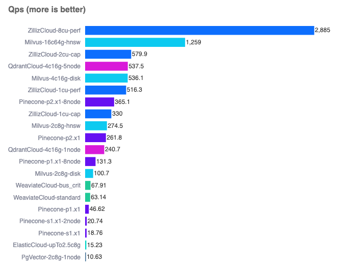
You can run a comparison yourself here.

Building The Pipeline

So here’s how the whole thing actually works in practice. When someone asks a question, we:

1. Store your ground truth in a vector database
2. Convert the user’s question into an embedding
3. Use cosine similarity (which is actually a pretty simple algorithm) to find matches
4. Pull back maybe the top 10 most relevant chunks of information

Now, there’s actually a whole science to storing these embeddings! It depends on stuff like:

• Which LLM you’re using
• The context window size you’re working with
• How much data you can throw at it before things get wonky

But honestly, these newer models with their huge context windows? They’ve made this SO much easier! You can throw a pretty big chunk of context at them, and they handle it like champs. No more worrying about degrading quality or hallucinations (well, mostly! 😅).

Practical Implementation Tips

When you’re actually implementing this, you want to:

1. Chunk your data into manageable sizes
2. Store references to your original documents
3. Fetch those reference docs when you get a match

This way, when your LLM is answering questions, it’s not just pulling from its training data - it’s using actual, accurate information from your knowledge base!

Below is a representation of how you could your RAG data using Postgres

documents

document_chunks

You know what’s cool about this setup? The metadata JSONB field is like this super flexible catch-all for whatever extra info you might need to track. This can become helpful for improving the relevance and accuracy of your search (more on that later on in the series). I usually stuff things in there like:

{
    "source_type": "technical_doc",
    "department": "engineering",
    "last_verified": "2024-01-18",
    "confidence": 0.95,
    "page_number": 42,
    "section": "API Documentation"
}

---

Next up, we’ll roll up our sleeves and implement a real world RAG solution against the MANEB syllabus - which can be used later to create a context aware AI tutor for Malawian Students!